Sensors and Transducers
A sensor is a device that measures or senses a number of physical properties and converts it into another analog quantity that can be measured electrically such as voltage, current, etc.
A transducer is a device that is connected to a sensor so as to convert the measured values into standard analog electrical signals such as 4 to20 mA. The output can be used directly by the system controller.
A transmitter is called to the combined package sensor and transducer. Some people use these terms interchangeably though it is not correct.
A pressure sensor is a device for the pressure measurement of gases or liquids. Pressure is an expression of the force required to stop a fluid from expanding and is usually stated in terms of force per unit area. A pressure sensor usually acts as a transducer; it generates a signal as a function of the pressure imposed.
The 4-20 mA current loop is the prevailing process control signal in many industries. It is an ideal method of transferring process information because the current does not change as it travels from the transmitter to the receiver. Since 4 mA is equal to 0% output, it is incredibly simple to detect a fault in the system.
Accuracy refers to how close measurements are to the “true” value, while precision refers to how close measurements are to each other. Accuracy describes the difference between the measurement and the part’s actual value and precision describes the variation we see when we measure the same part repeatedly with the same device.
Precision can be broken down further into two components: Repeatability: The variation observed when the same operator measures the same part repeatedly with the same device. Reproducibility: The variation observed when different operators measure the same part using the same device.
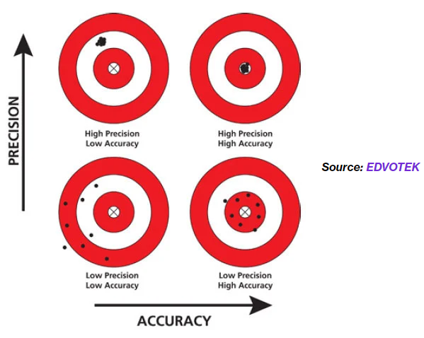
Figure 1: Differences between accuracy and precision
How data is read by controller:
We shall take a pressure sensor as our example to describe the process. The actual data is generated by the sensor. Pressure value mechanical deflection of a diaphragm, which is converted to electrical energy by a strain gauge (the diaphragm and strain gauge constitute a transducer), then to a numeric integer value by an input-output module of the controller.
The value can be stored somewhere from where our application reads the raw value. We have some reading for 3 similar pressure transmitters. Ideally when the current measurement is 4 milliamperes then the raw register reading should be 0 (ideal case). Since real-world objects are away from the ideal situations due to different reasons, so we need calibration. The sensor might behave or give different values at different conditions such as varying temperatures.
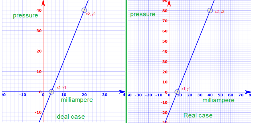
Figure 2: Ideal measurement, real measurement, and register values corresponds to 4 to 20 m amp (note the scale is different for both plot)
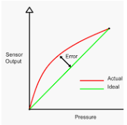
The above two images describe lots of the basics. In the left image, we have an ideal case and on the right side, we have a real case. We have an error in the sensor. It always shows a lower pressure value of the value corresponding to the electrical signal.
On the left side, at 20 milliamps current the pressure value is 40 bar (for example) but on the right side at 20 milliamps we see 30 bar. The slope of both curves is the same with a value of 2.5 (note see the scale is different for each curve).
For example on the left side, in the sensor we have a current of 10 milliamps and the sensor reading should be 15 but we are getting 5 (according to the picture on the right side)
For the ideal case, we can calculate the pressure value based on the following formula.
y = mx + c, where c is the intersection between point (0,0) and the y axis of the line. We can see that the line has crossed the y-axis at 0, -10. So the value of c is -10.
Exactly, in the same way, we can calculate the value of the pressure value based on the same formula but the intersection is in this case, -20.
So we can calculate the value of pressure value based on the measured current value.
How the value of m is calculated in the next section.
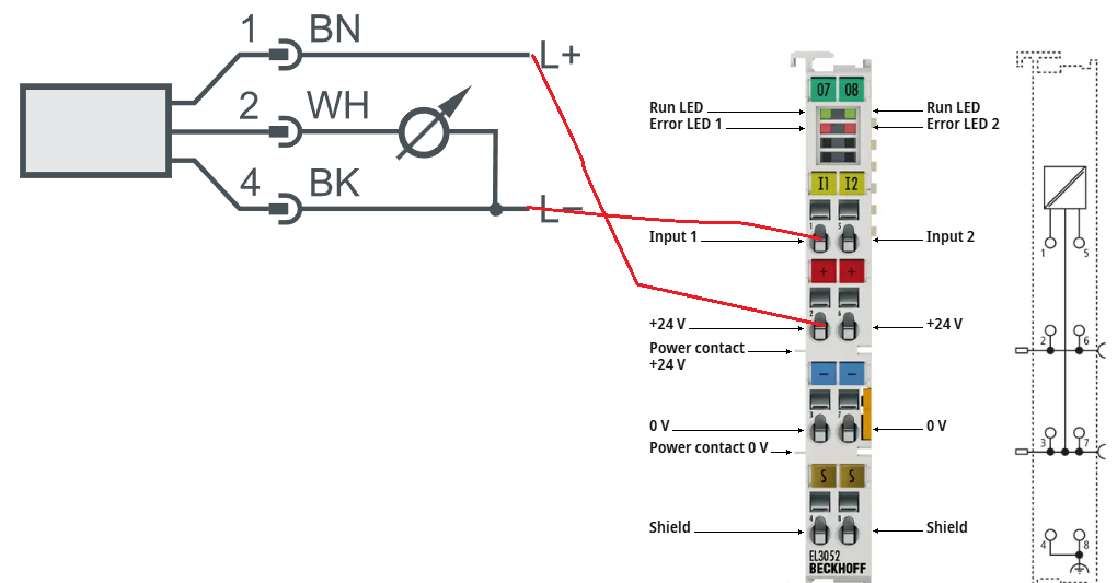
Pressure Sensor Connection
There are different variation or pressure sensors which can be connected to PLC. Here is a sample how this can be conected.
L+ goes to plus side of the card
L- goes to signal of the card.
Pressure Sensor Calibration :
As we see in the left-hand side image, the slope can have the same values as the actual case as compared with the ideal case.
Let’s say with a 4 milliamp value of the current we get an AD converted value of 0 and at 20 milliamps we get the AD converted value around 40. We can determine any pressure value the corresponding AD converted value by using the formula y = mx + c
If we know the value of x and c, then for any value of x (any value between 4 to 20), we can find the corresponding value of y (y axis value or pressure value). m is nothing but tan θ, where θ is the angle between the ideal line and the x-axis. m can be calculated by using the following formula where y2 is the maximum value of the y-axis (40) and y1 is the minimum value of the y-axis (0) and x2 is the maximum value of the x-axis (20) and x1 is the minimum value of x-axis (4).
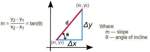
Figure 3: Slope calculation by using two points for a straight line
if we use the values, m = (40-0)/(20-4) = 2.5
Final formula is: y = 2.5x-10 (equation 1)
In the above equations, y is pressure value and x is the milliamps value. For each milliamps value we can find the pressure value.
In real case, if we observe the right side of the figure 2, we can see that slope is same but the intersection on y-axis is different. In this case, intersection is -20 (value of c).
Final formula is: y = 2.5x-20 (equation 2)
Offset Compensation:
Equation for ideal case: y = mx -10 => For a value of milliamps 10, we get pressure value, y = 2.5 * 10 -10 = 15
Equation for real case: y = mx -20 => For a value of milliamps 10, we get pressure value, y = 2.5 * 10 -20 = 5
Ideal case, the pressure value should be 15 but in a real pressure sensor, we get the value of 5. This is true for any measurement. How do we compensate for this?
Equation 1 and 2 can be re written like the following way:
y1 = mx -10
y2 = mx -20
y1-y2 = (mx-10) – (mx-20) => y1 = mx-10 -mx + 20 + y2
=> y1 = 10+y2, where y2 is the real measurement and y1 is the ideal measurement.
So for each measurement, we add 10 to the pressure sensor readings to get the actual measurement.
Slope Compensation:
For constant offset, we have seen that we can add or subtract a value from real measurement and we get the ideal value. That is a bit easy process to use it. But what when the actual curve has a different slope than the ideal one. It has deviated from the ideal one see the following figure.
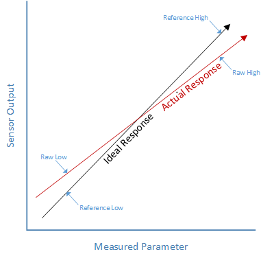
Figure 4: Ideal line is not parallel to the real line, m is not same and at the same time the offset value is different (ref 1)
As we see in Figure 4, the same technique will not work. We need to find a generic solution that works in both cases.
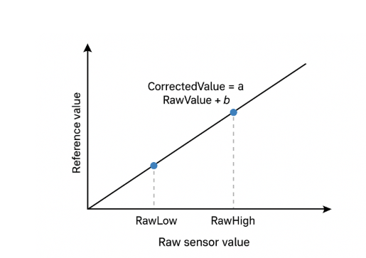
Figure 5: References Value VS Raw sensor value
If we plot the Raw sensor value in the X axis and the Corrected value in the Y axis, we shall have a linear equation.
CorrectedValue=a×RawValue+b
If we know the value of a and b, then for each on the line, we can find the reference value for each raw value.
We shall take two measurements: One near the low end of the measurement range and one near the high end of the measurement range.
You have two known calibration points:
| Raw Reading | True (Reference) Value |
|---|---|
| RawLow | ReferenceLow |
| RawHigh | ReferenceHigh |
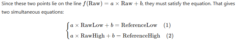
If we subtract 2 equations, we can find the value of a = (ReferenceHigh−ReferenceLow)/(RawHigh−RawLow)
This is the slope of the calibration line.
Now we can find the value of b by substituting a into equations 1 or 2, and find the corrected value:
CorrectedValue = ((RawValue – RawLow) * ((ReferenceHigh−ReferenceLow)/(RawHigh−RawLow)) + ReferenceLow
By this equation, we can calculate actual values for each point:
double CorrectedValue;
double RawValue = 16000 ;
double RawLow = 6000;
double RawHigh = 28000;
double ReferenceLow = 8000;
double ReferenceHigh = 29000;
double RawRange = RawHigh – RawLow;
double ReferenceRange = ReferenceHigh – ReferenceLow;
CorrectedValue = (( (RawValue – RawLow) * ReferenceRange) / RawRange) + ReferenceLow;
With these values, CorrectedValue is: 17545
4-20 mA Current Loop
References:
=> https://learn.adafruit.com/calibrating-sensors/two-point-calibration
=> https://www.azosensors.com/article.aspx?ArticleID=723
=> https://control.com/textbook/instrument-calibration/zero-and-span-adjustments-analog-instruments/
=> https://instrumentationtools.com/pressure-switch-calibration/
=> https://www.instrumentationtoolbox.com/2012/12/understanding-instrument-calibration.html